Two minimal single-event laser-cavitation models
Problem, architecture and scope
Model A calculates source pressure and first-ejection outlet speed. It uses specified source work, gas volume and liquid inventory. It also derives their energy ceilings. Model B adds hydrogel compliance and loss. It calculates gel load and the remaining emitted output.
An initially spherical chamber contains gas and carrier liquid. A liquid outlet already connects it to the surroundings. Initially connected chamber liquid sets the finite discharge budget. Effective channel inertance is a separate input. Model A fixes the chamber wall. Model B surrounds it with intact, undrained spherical hydrogel. Gas expansion enlarges the chamber or displaces liquid through the outlet. The sealed control fixes outlet motion at zero. This architecture describes expansion-driven external ejection. Collapse jets and gel penetration require different models.
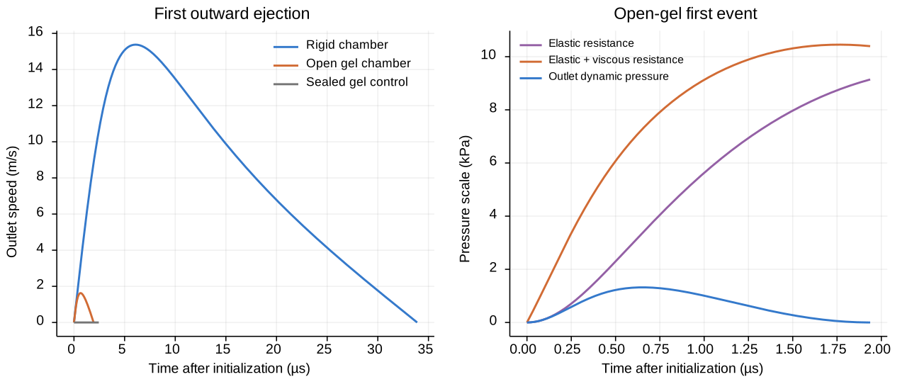
A single 10 ns optical pulse is represented by post-activation initial data. Time zero follows activation and pressure equilibration. Optical heating, nucleation and energy conversion are excluded. There is no periodic load. Follow the first outward ejection until speed returns to zero. Stop sooner if liquid exhausts or a validity screen triggers. The sealed control stops at its first wall turning point. Evaluate speed maxima within these episodes. Later collapse and rebound are excluded.
Time starts at the initialized post-activation state. Positive outlet velocity points outward. Discharge coordinate means emitted volume divided by outlet area. Positive radial direction runs from chamber center into gel. Positive wall velocity means expansion. Ambient pressure is constant and absolute. Initially, the wall is stress-free relative to ambient. All initial mechanical velocities are zero. Chamber pressure is uniform. Gas-pocket shape and internal gas/liquid tension are neglected. The external meniscus supplies capillary resistance. Far-field radial stress tends to negative ambient pressure. Far-field displacement decays. The outlet exits at ambient with the specified meniscus pressure. An open case requires an existing channel. The sealed case emits zero liquid.
Constitutive assumptions. The source is a closed adiabatic ideal gas. Its exponent is constant. A PFC-vapor EOS is outside this control. Liquid and undrained gel densities are constant. The column has fixed effective inertance and a finite discharge budget. Gel elasticity is incompressible neo-Hookean with Kelvin–Voigt viscosity. Optional port losses are linear and quadratic. Outlet focusing, free-surface shape, fracture, phase exchange and diffusion remain unresolved. The spherical gel law approximates a chamber with a small outlet. Planar-layer mechanics requires a separate model. Material predictions require calibration.
Start from the first law, volume conservation and unsteady Bernoulli. Add the specified source EOS and spherical gel constitutive model. The course explains mechanisms and finite-energy budgets. Chapters 1–3 and Appendix A supply these model blocks. Brennen, Chapter 2 discusses spherical momentum and polytropic assumptions. The gas-volume coupling, finite-stroke rule and diagnostics are derived here.
Symbol glossary and conventions
All lengths use m, times s, masses kg, pressures Pa, energies J and forces N. Subscripts 0 and ref label initial and unstressed states; g, j, el, cap, dis and obs label gas, emitted jet, elastic, capillary, dissipative and observer quantities. Superscripts on scalar quantities are powers. A dot is a derivative in time. An integral is over the displayed real variable or surface. Absolute value is scalar magnitude. A hat labels the normalized state defined below. The constant pi is dimensionless. Arithmetic has its usual real meaning. No scalar is reused for a different role.
| Symbol | Meaning and restrictions | Unit |
|---|---|---|
| Time after the initialized post-activation state | s | |
| Discharged volume divided by outlet area, and outlet speed | m, m/s | |
| Chamber radius and wall velocity; | m, m/s | |
| Unstressed chamber radius and initial gas-pocket radius | m | |
| Outlet radius, effective inertance length, discharge-budget length, and area | m, m, m, m² | |
| Current gas, initial gas, initial chamber, and ambient-equilibrium gas volumes | m³ | |
| Current absolute source, initial absolute source, and absolute ambient pressures | Pa | |
| Constant adiabatic ideal-gas exponent, strictly greater than one | dimensionless | |
| Gas internal energy and available adiabatic expansion work relative to ambient | J | |
| Carrier density, undrained gel density, and effective liquid-column inertia mass | kg/m³, kg/m³, kg | |
| Effective surface tension, meniscus resistance, and reversible meniscus work | N/m, Pa, J | |
| Fitted linear port resistance, dimensionless quadratic loss coefficient, dissipative port pressure | Pa s/m, dimensionless, Pa | |
| Outlet flag: one for an open channel, zero for sealed | dimensionless | |
| Positive gel shear modulus and nonnegative effective network viscosity | Pa, Pa s | |
| Current gel radial coordinate, reference radial coordinate, dummy radius in a work integral | m | |
| Radial stretch, either equal tangential stretch, and change-of-variable ratio | dimensionless | |
| Radial/tangential elastic Cauchy stress and incompressibility multiplier | Pa | |
| Elastic wall resistance and elastic-plus-viscous wall resistance | Pa | |
| Column kinetic energy, gel kinetic energy, elastic work, irreversible losses, emitted energy | J | |
| Irreversible port and gel powers | W | |
| Axial resultant of elastic resistance on one chamber hemisphere | N | |
| Polar angle about the outlet axis and solid-angle element | dimensionless | |
| Velocity, time and emitted-impulse normalization scales | m/s, s, N s | |
| Seven normalized motion and accounting states | dimensionless | |
| Energy residual divided by available work | dimensionless | |
| Emitted RMS speed, outlet dynamic-pressure scale, emitted impulse, emitted mass | m/s, Pa, N s, kg | |
| Declared observer area, averaging interval and mean arrest-pressure bound | m², s, Pa | |
| Matched peak-speed, emitted-energy, emitted-impulse and peak dynamic-pressure ratios | dimensionless | |
| Reference communication speed, path length, communication ratio, liquid/wall Mach diagnostics | m/s, m, dimensionless |
| | Streamline coordinate and inlet/outlet positions | m | | | Local speed, fixed area-ratio profile, and local cross-sectional area | m/s, dimensionless, m² | | | Gas internal energy plus work against ambient, referred to initial volume | J |
Step 1 — Conserve volume and declare the finite source
Eq. (E01) — geometric identities.
Symbols before Eq. (E01): is outlet area (m²); is outlet radius (m); are initial gas, initial chamber and current gas volumes (m³); are initial gas, reference chamber and current chamber radii (m); is discharged volume divided by area (m); is discharge-budget length (m); pi is dimensionless.
The second row conserves chamber liquid volume. Gas gains discharged liquid volume and chamber expansion volume. Model A fixes chamber expansion at zero. Stop when the finite liquid discharge budget is exhausted.
Eq. (E02) — initial data and admissible outward stroke.
Symbols before Eq. (E02): are lengths (m); are liquid and wall speeds (m/s); are positive reference radius and discharge-budget length (m); is area (m²); are initial volumes (m³); argument zero labels initialization.
Zero initial speeds are specified post-activation inputs. Nucleation is excluded. The finite stroke bounds discharged mass.
Eq. (E03) — adopted ideal-gas energy and adiabatic first law.
Symbols before Eq. (E03): is internal energy (J); is absolute source pressure (Pa); is gas volume (m³); is the constant ideal-gas exponent; denotes a differential along the closed adiabatic source trajectory.
The first relation defines the source constitutive model. The second applies its adiabatic first-law balance. Heat and mass exchange vanish after initialization. Differentiate the first relation. Multiply by the exponent minus one to obtain the third. Condensation and further PFC vapor production are excluded.
Eq. (E04) — integrate the pressure law.
Symbols before Eq. (E04): are positive current and initial absolute pressures (Pa); are positive current and initial volumes (m³); is dimensionless; is the logarithm of a dimensionless ratio; is a trajectory differential.
Collect the differential terms in Eq. (E03). Divide by positive pressure and volume. Integrate from the initial state to fix the constant. Exponentiation gives the pressure law. Expansion lowers pressure. No periodic source is prescribed.
Step 2 — Compute the finite work budget
Eq. (E05) — ambient equilibrium and available expansion work.
Symbols before Eq. (E05): are gas volumes (m³); are initial source and ambient absolute pressures (Pa); is dimensionless; is available adiabatic expansion work (J); is a dummy positive gas volume (m³); the integral is along the declared pressure-volume path.
Apply Eq. (E04) at ambient pressure. Take the positive root to find equilibrium volume. Integrate overpressure to define available work. Integrate the volume power, whose exponent differs from one. Evaluate both endpoints and factor the initial volume. Pressure times volume has units J. Numerically invert this monotone relation for initial pressure. Changing the work budget changes the initial state. It adds no later work.
Available work means post-activation mechanical availability. Incident optical energy is a separate quantity. Determine available work from a measured pressure-volume path. Alternatively, use absorbed energy with a supported conversion and phase model. Source mass and phase composition must support the initialized state. Conversion efficiency and PFC EOS remain unspecified.
Eq. (E05a) — uniqueness of the finite-work inversion.
Symbols before Eq. (E05a): is available work (J); are initial and ambient pressures (Pa); are initial, equilibrium and dummy gas volumes (m³); is dimensionless; fixes initial volume, ambient pressure and exponent; denotes the indicated pressure limit.
Apply Leibniz differentiation in the first row. The endpoint pressure equals ambient, so its term vanishes. Integrate the remaining positive power for the second row. Equal source and ambient pressures give zero work. Equilibrium-volume terms grow sublinearly at large source pressure. This gives the final limit. Positive available work therefore selects a unique initial pressure.
Step 3 — Accelerate an outlet flow and retain actual emitted output
Eq. (E06) — inertia, capillary resistance and port loss.
Symbols before Eq. (E06): is effective column inertia mass (kg); is carrier density (kg/m³); is outlet area (m²); are inertance length and outlet radius (m); are pressures (Pa); is tension (N/m); is fitted resistance (Pa s/m); is dimensionless; is outlet speed (m/s); absolute value denotes magnitude.
Column inertia and emitted mass are separate quantities. The meniscus model assumes a pinned hemisphere. Different curvature requires different entry pressure. Measure or fit the linear resistance. Steady Poiseuille resistance needs justification for this short event. The odd-in-speed loss dissipates energy in either direction.
Meniscus pressure stays constant during this episode. Its integral is work against a constant conservative load. The model excludes evolving free-surface energy. Persistent hemispherical curvature during jet formation is not established. Changing curvature, contact-line motion or breakup requires a revised entry model.
Eq. (E06a) — derive inertance and the outgoing kinetic head.
Symbols before Eq. (E06a): are streamline coordinate and inlet/outlet positions (m); is local speed and outlet speed (m/s); is a fixed dimensionless profile; are outlet and local areas (m²); is inertance length (m); is density (kg/m³); is pressure (Pa); is time (s); are fixed-position derivatives; a dot is a time derivative. The large-reservoir approximation sets inlet speed to zero and outlet profile to one.
Fixed-geometry continuity gives the first velocity profile. The second row applies inviscid streamline Euler momentum. Integrate the fixed profile to obtain inertance. Integrate convection to obtain endpoint kinetic heads. Neglect reservoir inlet speed and retain outlet head. Substitute the continuity area relation in the energy integral. This yields the same inertance length. The approximation represents an existing channel. Free-surface focusing and transverse kinetic energy are excluded. Calibrate effective inertance and loss for the actual geometry.
Eq. (E07) — unsteady Bernoulli and the explicit outlet flag.
Symbols before Eq. (E07): is discharged volume divided by outlet area (m); is outward outlet speed (m/s); dots are time derivatives; is the open/sealed flag; is density (kg/m³); is inertance length (m); are source, ambient, meniscus and dissipative pressures (Pa).
Integrate the pressure gradient in Eq. (E06a). Add the specified meniscus and dissipative pressure drops. Divide by positive density and inertance length. This gives outlet acceleration. A sealed outlet retains its zero initial speed. The kinetic-head term accounts for energy leaving the outlet.
Eq. (E08) — column storage and dissipative power.
Symbols before Eq. (E08): are stored energies (J); is effective inertia mass (kg); is outlet speed (m/s); are pressures (Pa); is area (m²); is discharge volume divided by area (m); is dissipative power (W); is resistance (Pa s/m); is density (kg/m³); are dimensionless; is a time derivative.
Differentiate stored energy and insert Eq. (E07). Add meniscus work to cancel the meniscus pressure term. Dissipative pressure times flow rate gives dissipative power. The final kinetic-head term gives emitted power. Column storage and irreversible loss remain separate.
Eq. (E08a) — finite emitted mass, energy and impulse.
Symbols before Eq. (E08a): is emitted mass (kg); is discharged kinetic energy (J); is discharged axial impulse (N s); is density (kg/m³); is area (m²); is discharge volume divided by area (m); is nonnegative outlet speed (m/s); is the outlet flag; dots are time derivatives and argument zero labels initialization.
Multiply mass flow by specific kinetic energy for emitted power. Multiply it by axial speed for emitted impulse rate. Integrate each rate over time. Column energy and momentum describe instantaneous storage. Emitted energy and impulse describe discharged output.
Step 4 — Retain only the gel mechanics needed for confinement
Eq. (E09) — incompressible spherical mapping and principal stretches.
Symbols before Eq. (E09): are current material radius, reference material radius, current wall radius and reference wall radius (m); are dimensionless radial and tangential stretches; differentiates at fixed time; and .
Equate reference and current material volumes outside the wall. Differentiate that mapping for the second row. Use radial and tangential length ratios for the third. Their product checks local volume conservation.
Eq. (E10) — declared neo-Hookean stress and radial equilibrium.
Symbols before Eq. (E10): are radial/tangential Cauchy stress and an incompressibility multiplier (Pa); is shear modulus (Pa); are stretches; are material radii (m); is a radial derivative (Pa/m).
The first row is the adopted constitutive law. Subtract the stresses to eliminate constraint pressure. The third row states spherical elastic equilibrium. Its integral gives elastic resistance. Radial inertia and viscosity are added separately below.
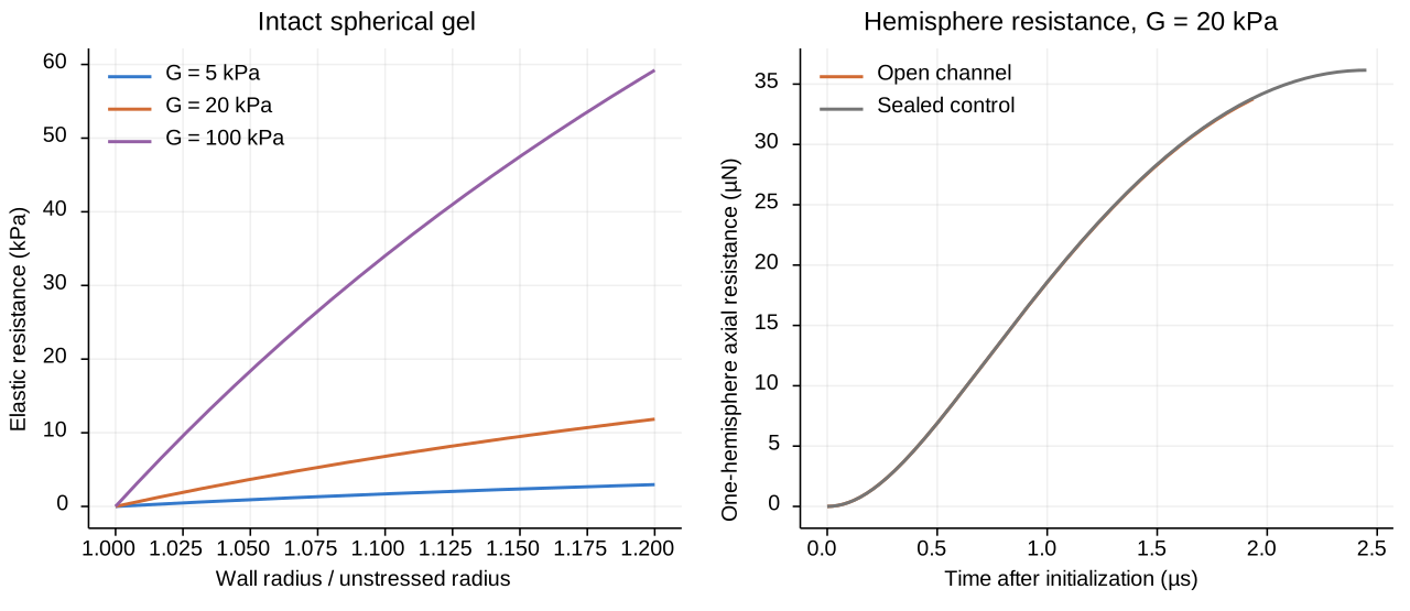
Eq. (E11) — evaluate the spherical elastic resistance.
Symbols before Eq. (E11): is elastic resistance pressure (Pa); is shear modulus (Pa); are radii (m); is a positive dimensionless integration variable; denotes a differential; the radial integral uses the infinite-medium stress boundary condition.
Integrate the stress difference in Eq. (E10). Differentiate the volume mapping at fixed wall radius. Substitute it to obtain the third row. Factor the difference of squares and cancel the common factor. The wall endpoint is reference radius divided by current radius. The far-field endpoint is one. Integrate the polynomial and evaluate both endpoints. The last two rows recover Appendix A, Eq. (A-E05). No wave field is required.
Eq. (E12) — integrate the recoverable gel work.
Symbols before Eq. (E12): is elastic work (J); is shear modulus (Pa); are current wall, reference wall and dummy wall radii (m); is the pressure from Eq. (E11) evaluated at the dummy radius (Pa); pi is dimensionless.
The first row integrates traction against spherical volume change. Insert Eq. (E11) and integrate each power. Evaluate both endpoints. The lower endpoint is two-thirds of the reference-radius cube. Modulus times volume gives J. This energy is recoverable elastic storage.
Eq. (E13) — gel resistance checks.
Symbols before Eq. (E13): is pressure (Pa); is energy (J); is modulus (Pa); are lengths (m); is radius differentiation; denotes terms of the indicated small-displacement order; is the stated radius limit.
Substitute the unstressed radius to check the reference state. Differentiate work to check traction. Taylor expansion gives positive small-strain stiffness and quadratic stored work. Infinite radius ratio gives a pressure plateau. Work still grows with volume. Damage tolerance and useful jet formation are not established.
Step 5 — Add radial inertia and viscous loss
Eq. (E14) — spherical radial kinetic energy and Newtonian gel loss.
Symbols before Eq. (E14): is radial gel kinetic energy (J); is density (kg/m³); are wall radius and speed (m, m/s); is spatial radius (m); is network viscosity (Pa s); is irreversible power (W); are wall resistance pressures (Pa); pi is dimensionless.
The volume mapping gives radial velocity. Squaring it produces a convergent reciprocal-square radial integral. Use the appendix Kelvin–Voigt coefficients, Eqs. (A-E09)–(A-E12). Viscosity opposes both directions of wall motion. Its dissipated power is nonnegative. Radiation and wave-field losses are excluded.
Eq. (E15) — radial motion and its energy identity.
Symbols before Eq. (E15): are wall radius and speed (m, m/s); dots are time derivatives; is density (kg/m³); are pressures (Pa); is viscosity (Pa s); are energies (J); is power (W); pi is dimensionless.
The first row adopts undrained spherical momentum balance. Initial elastic overpressure is zero. Differentiate kinetic energy in Eq. (E14) using the product rule. Substitute wall kinematics to obtain the second row. Multiply the first row by volume rate. Insert elastic work from Eq. (E13). Insert viscous power from Eq. (E14) for the third row. Model A fixes radius, eliminating radial kinetic and elastic storage.
Eq. (E16) — a defined confinement force.
Symbols before Eq. (E16): is axial force on one hemisphere (N); is uniform spherical elastic resistance (Pa); is radius (m); is polar angle measured from the outlet axis; pi is dimensionless; the integral projects traction onto that axis.
This force is the directional resultant on one hemisphere. The complete sphere has zero resultant by symmetry. Integrating pressure magnitude over a sphere gives a different quantity. A target patch requires its own area and load path.
Step 6 — Close and audit the combined energy balance
Eq. (E17) — total source volume rate and accumulated loss.
Symbols before Eq. (E17): is gas volume (m³); is area (m²); are speeds (m/s); is radius (m); is the open/sealed flag; is accumulated loss (J); are powers (W); dots denote time derivatives.
Differentiate Eq. (E01) and insert both kinematic relations. Add port and gel dissipation from their separate motions.
Eq. (E18) — explicit cancellation of source-to-receiver work.
Symbols before Eq. (E18): are stored, lost and emitted energies (J); are pressures (Pa); is gas volume (m³); is area (m²); are speeds (m/s); is radius (m); is dimensionless; is a time derivative; pi is dimensionless.
Combine the source first law, Eq. (E03), with column storage, Eq. (E08). Add radial storage, Eq. (E15), and accumulated loss, Eq. (E17). Each dissipative power cancels its loss accumulator. Emitted kinetic power cancels Eq. (E08a). Substitute volume rate to cancel the remaining source exchange. One evolving source pressure closes this balance. An independently prescribed radius history would break it.
Eq. (E19) — numerical acceptance residual.
Symbols before Eq. (E19): is dimensionless residual; are pressures (Pa); are volumes (m³); is dimensionless; are stored, lost, emitted and available energies (J), with strictly positive available work.
Subtract initial stored energy from Eq. (E18), then normalize. Include gel kinetic and elastic storage. A near-zero residual checks numerical conservation. EOS and geometry calibration require separate evidence.
Step 7 — Map the equations to native COMSOL states
Eq. (E20) — normalization definitions.
Symbols before Eq. (E20): is speed scale (m/s); is time scale (s); is impulse scale (N s); are lengths (m); are speeds (m/s); is effective column mass (kg); are losses, emitted energy and available work (J); is emitted impulse (N s); seven hatted states are dimensionless normalized quantities.
Normalization changes scales without changing the model. Native states are qq, vv, rr, ww, dd, ee, ii. Model A excludes two radial states, leaving five scalars. Model B uses seven. Three accumulate loss, emitted energy and emitted impulse.
Eq. (E21) — dimensionless residuals integrated in physical time.
Symbols before Eq. (E21): all hatted states are dimensionless; their dots differentiate in physical time (1/s); is time (s); is the outlet flag; are speeds (m/s); are lengths (m); are densities (kg/m³); are pressures (Pa); is viscosity (Pa s); are powers (W); is work (J); is area (m²); is impulse scale (N s).
Insert Eq. (E20) into motion and accounting equations. Divide speed derivatives and accumulated quantities by their respective scales. Multiply each row by the time scale. Every residual is dimensionless. Model A fixes the wall and excludes radial rows. Total gas volume determines algebraic source pressure.
Step 8 — Bound defined velocities, emitted output and pressure observers
Eq. (E22a) — show the minimum of source mechanical potential.
Symbols before Eq. (E22a): is source internal energy plus work against ambient, referenced to initial volume (J); is internal energy (J); are positive pressures (Pa); are volumes (m³); is dimensionless; is available work (J); derivatives are with respect to positive gas volume.
The source first law gives the first derivative. Differentiate Eq. (E04) for the second. Strict convexity gives a unique global minimum at ambient pressure. Evaluate the potential difference to obtain Eq. (E05). This establishes the work budget within the adopted control.
Eq. (E22) — separate outlet-speed and emitted-RMS ceilings.
Symbols before Eq. (E22): are column kinetic energy, emitted energy and available work (J); is effective column inertia mass (kg); is actual emitted mass (kg); is outlet speed (m/s); is emitted mass-weighted RMS speed (m/s); is outlet dynamic-pressure scale (Pa); is density (kg/m³); are outlet area and inertance length (m², m); square roots are nonnegative.
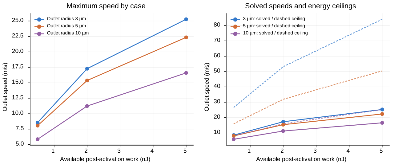
Every listed receiver energy is nonnegative on the outward branch. Combine Eq. (E18) with the minimum in Eq. (E22a). Isolate column kinetic energy and divide by positive effective mass. This gives the outlet-speed ceiling. Emitted energy and positive emitted mass define the RMS ceiling. Insert column mass from Eq. (E06) for the dynamic-pressure ceiling. The outlet ceiling depends on effective inertance. The emitted-RMS ceiling follows from conservation and specified mass. Liquid exhaustion may stop the trajectory before either ceiling.
A finite energy budget needs a positive mass lower bound. Without it, a universal RMS-speed maximum cannot be computed. A pointwise pressure maximum needs a contact or compression model. Missing: area, duration and load path. Source pressure, outlet dynamic pressure and observer pressure are distinct quantities.
Eq. (E23) — finite emitted impulse and a mean arrest-pressure bound.
Symbols before Eq. (E23): is emitted impulse (N s); is emitted mass (kg); is a dummy cumulative emitted-mass coordinate (kg); is the same outlet-speed history reparameterized by discharged mass (m/s); are emitted energy and available work (J); is positive observer area (m²); is positive averaging time (s); is mean positive arrest pressure attributable to these emitted parcels (Pa).
Apply Cauchy–Schwarz to the integrable finite speed history. Its two integrals are emitted mass and twice emitted energy. Assume parcels stop without reversal and receive no extra actuation. Their received impulse is then bounded by incoming impulse. Divide by specified area and duration for mean pressure. Defaults are outlet area and one microsecond. Instantaneous impact pressure remains uncomputed. Propagation and water hammer are excluded.
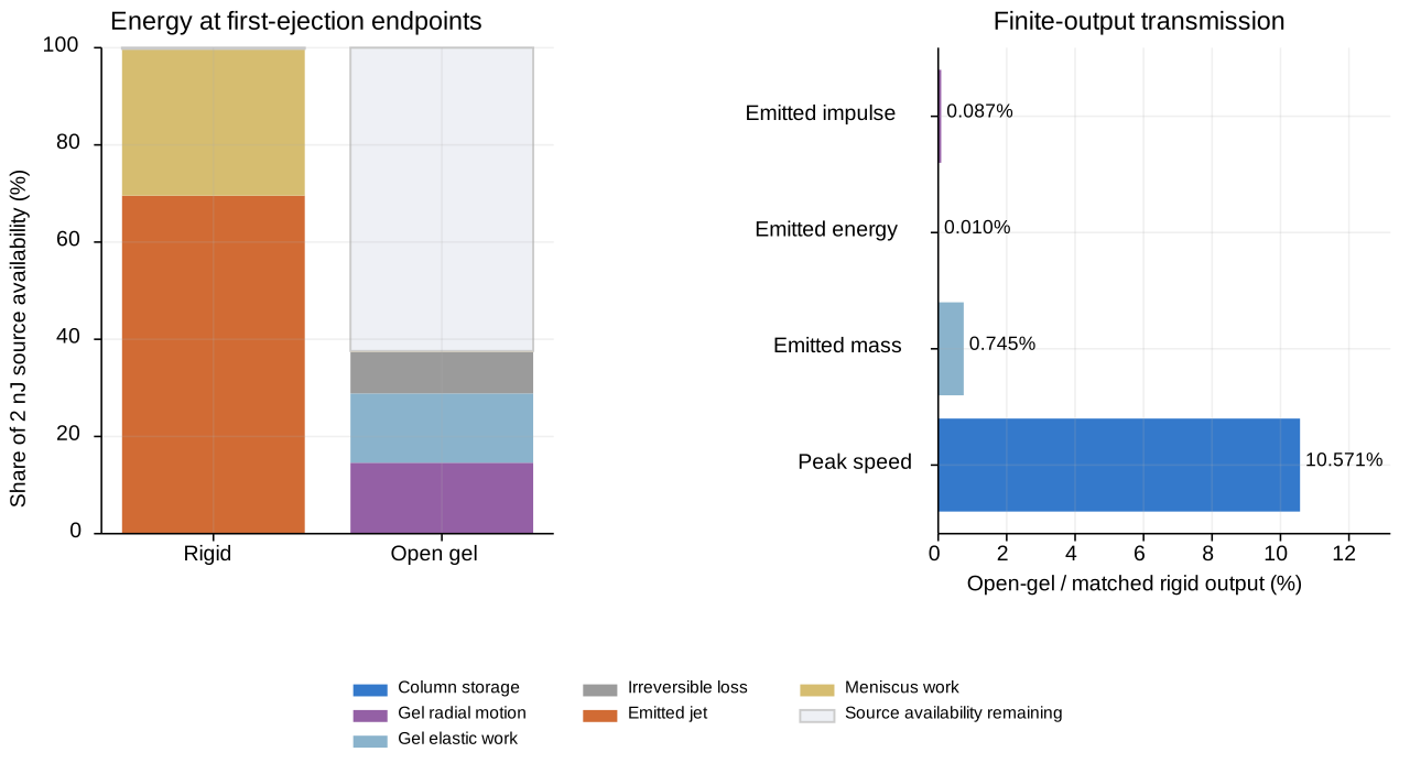
Eq. (E24) — matched single-event transmission measures.
Symbols before Eq. (E24): are dimensionless ratios; subscripts identify matched rigid and hydrogel cases with the same source state, density and outlet geometry; are first-event outlet-speed maxima (m/s); are emitted energies accumulated by each event endpoint (J); are emitted impulses (N s); are first-event dynamic-pressure maxima (Pa); denominators are positive in the rigid reference.
At equal density, dynamic-pressure ratio equals speed ratio squared. Integrate full histories for emitted energy and impulse. A peak speed cannot determine these integrals. Stop each open case at speed return, inventory exhaustion or validity screen. Matched cases may therefore have different endpoints. These ratios compare finite outputs per shot. They are distinct from frequency-domain transfer functions. Every emitted-output ratio is zero for a sealed channel.
Step 9 — Declare the regime and check its communication rate
Eq. (E25) — communication and Mach diagnostics.
Symbols before Eq. (E25): are dimensionless diagnostics; is communication length (m), chosen as inertance length for A and the greater of inertance length and chamber diameter for B; is reference speed (m/s); is positive absolute pressure (Pa); is its time derivative (Pa/s); is dimensionless; are volume and its rate (m³, m³/s); are speeds (m/s); absolute values denote magnitudes.
Logarithmically differentiate Eq. (E04) for the second communication expression. Compare pressure-change and pressure-communication times. No propagation field is solved. The open baseline communication diagnostic stays below 0.1. This is a stipulated screen, whose error bound remains unvalidated. Both Mach diagnostics must also stay below 0.1.
Undrained behavior requires events much shorter than solvent drainage. The course uses an illustrative 30 micrometer drainage scale. Its estimated drainage time is 1.5 s. These events last microseconds. Actual permeability and rate-dependent moduli remain unmeasured. Check small-outlet geometry, positive liquid inventory and intact gel. Check gas breakthrough before the finite stroke ends. The 20% stretch stop is a stipulated deformation screen. Measured fracture strain is missing.
Check the sealed case communication ratio separately. Energy conservation cannot resolve failed pressure communication. A pressure-history prediction requires that screen to pass.
What the completed models can establish
The models provide conditional first-event solutions and maxima. They derive energy ceilings, spherical gel resistance and recoverable work. They also calculate matched finite-output ratios. A universal cavitation maximum is not established. Calibrated PFC limits and the excluded 10 ns activation pressure remain unresolved. Collapse-jet maxima and transmission through intact gel also remain unresolved.
Experimental validation requires post-activation phase volume and pressure. A measured pressure-volume path can supply the source work. Record absorbed pulse energy and conversion evidence. Specify moving liquid mass, outlet geometry and channel status. Measure gel modulus and viscosity at the event strain rate. Measure cavity volume, emitted speed, mass and wall deformation together. Declare comparison locations and averaging intervals. Compare source pressure, dynamic pressure and all four finite-output ratios.